|
Shock-turbulence interaction
The scientific understanding of
shock/turbulence interactions remains limited, despite decades of
efforts. The most fundamental problem is arguably that of isotropic
turbulence passing through a nominally normal shock wave, termed
`canonical shock/turbulence interaction' in this report. This problem
has received considerable attention in past theoretical, experimental, and computational
studies. The linear theory by Ribner (NACA report, 1953 predicts that the velocity and vorticity variances
are amplified during the shock interaction, and that there is an
inviscid adjustment region behind the shock where turbulence adjusts
to its post-shock state. This theory is formally valid in the limits
of infinite Reynolds number and zero turbulent Mach number, but has
thus far (Lee et al., J. Fluid Mech. 1993; 1997) only been tested at Reynolds numbers
of Re_l=20. At these low Reynolds numbers, the viscous
decay behind the shock is comparable to or larger than the inviscid
adjustment, which makes direct comparisons to the linear theory
difficult. Furthermore, the spectrum of turbulence is not truly
broadband at such Reynolds numbers. And, finally, there is reason to
believe that previous studies have not truly resolved the dissipative
motions of the turbulence.
The Hybrid code
(Larsson et al., CTR
Annual Research Briefs 2007) solves the compressible Navier-Stokes
equations for a perfect gas using solution-adaptive finite-difference
schemes on Cartesian (but stretched) grids. Near shock waves or other
discontinuities, a 5th order accurate weighted essentially
non-oscillatory (WENO) scheme is used. In these
regions, the equations are discretized in divergence (or conservative)
form, thereby ensuring convergence to the correct weak solution. Away
from shock waves, a 6th-order accurate central difference scheme is
used. This scheme has nominally zero numerical dissipation, which is
an important
attribute for the prediction of broadband turbulence. The coupling of the different discretizations globally conserves mass, momentum, and energy, and was
shown to be linearly stable. The semi-discrete
system is integrated in time using classic 4th-order, fully explicit Runge-Kutta. The method is implemented using C++, and parallelized
through domain decomposition with communication handled by MPI.
The code has been run on several machines.
|
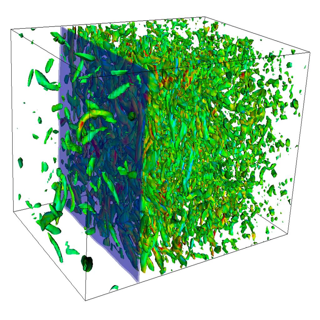
Figure 1. Snapshot of
shock/turbulence interaction at M=2, Mt=0.15, Re_l = 40. The flow
is from left to right, with the shock visualized by transparent
isosurfaces of compression. Vortex cores are visualized by
isosurfaces of the second invariant of the velocity gradient
tensor, colored by the vorticity magnitude. |
The essence of shock/turbulence
interaction is shown in Figure 1. The incoming
turbulence is isotropic, as evidenced by the random orientation of the
vortex cores. The shock compresses the turbulence in the x
direction, increasing the vorticity and making the post-shock
turbulence axisymmetric with vortex cores predominantly oriented in
the y-z plane.
|
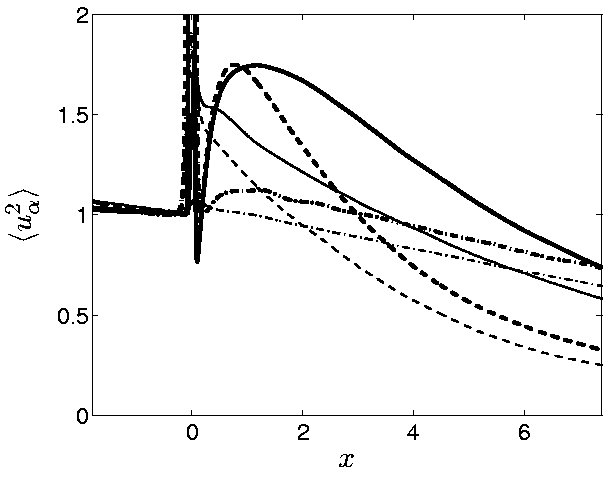
Figure 2. Streamwise (thick) and
transverse (thin) Reynolds stress for canonical shock/turbulence
interaction. Variance of Reynolds stress and vorticity for
(M,M_t)=(2.0,0.15) (solid), (M,M_t)=(2.0,0.30) (dashed), and (M,M_t)=(1.1,0.15)
(dash-dotted). |
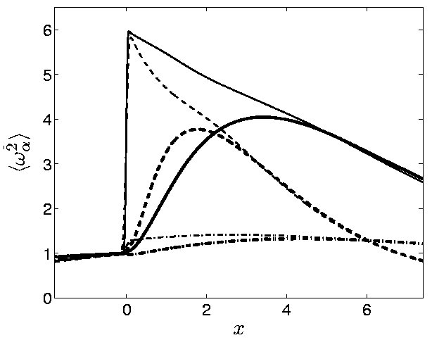
Figure 3. Streamwise (thick) and transverse (thin) vorticityfor
canonical shock/turbulence interaction. Variance of Reynolds
stress and vorticity for (M,M_t)=(2.0,0.15) (solid), (M,M_t)=(2.0,0.30)
(dashed), and (M,M_t)=(1.1,0.15) (dash-dotted). |
The variances of velocity and vorticity
fluctuations are shown in figures 2-3 for a sequence of cases. The
transverse vorticity is directly amplified at the shock due to the
compression, while the streamwise vorticity is initially unchanged.
Behind the shock, the out-of-equilibrium turbulence adjusts towards
an isotropic state, although the Reynolds stresses never reach
isotropy in these runs. One outstanding question in
shock/turbulence interaction is whether the turbulence truly returns
to isotropy. The relatively low Reynolds number of the present (and
all
previous) runs implies a quick viscous decay behind the shock, which
overwhelms any return-to-isotropy. Large-scale calculations at
higher Reynolds numbers are needed to illuminate this issue.
|
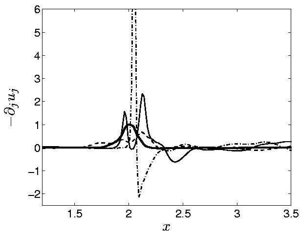
Figure 4. Compression for canonical shock/turbulence interaction.
Instantaneous (thin) and average (thick) profiles
of compression (negative dilatation) and density for (M,M_t)=(1.1,0.15).. |

Figure 5. Density for Canonical shock/turbulence interaction.
Instantaneous (thin) and average (thick) profiles
of compression (negative dilatation) and density for (M,M_t)=(1.1,0.15).. |
At high enough turbulent Mach number, M_t, the turbulent pressure
fluctuations become comparable to the pressure jump associated with
the shock, which significantly alters the instantaneous shock
profile. Some instantaneous profiles of the compression (negative
dilatation) and density along the x axis are shown in figures 4-5 for
such a case. The instantaneous structure of the shock varies wildly,
from being twice as strong as on average, to being replaced by a
smooth compression wave, to being replaced by two weaker shocks. This
intermittency is largely absent at lower values of M_t, and represents
a second outstanding fundamental question in shock/turbulence
interaction. In fact, the regime of high-M_t shock/turbulence interaction
remains largely unexplored in the literature.
|